Index |
Last Chapter |
Next Appendix |
A fundamental feature of a simulator modelling moving objects must obviously be how it handles collisions and interactions. And in order to do this, it must first of all determine whether a collision has occurred between a pair of objects.
The normal, and most straightforward way, of handling this problem is to simply simulate the movement of the objects, and calculate mathematically whether they overlap. If they do overlap, a collision has occurred.
Unfortunately, this is not entirely practical at the nanoscale. The difficulty lies in the fact that particles are not moving in straight lines, rather they are following a Brownian motion random-walk that are approximated as a Gaussian probability distribution. The scale of the simulation could be altered to the level where the particles were (effectively) moving in straight lines, but this would involve modelling the objects in picoseconds and picometres, which is unsustainable. Such modelling is already done, and quite widely, but is many orders of magnitude too slow for examining the interactions of large groups of macro-molecules.
The approach taken here is to calculate the odds of the particles colliding, and then to randomly determine whether or not they did collide. Determining the odds of collision turns out to be a challenging task.
The problem fundamentally is "With two spheres of given radius, with given standard deviations of movement, at a certain separation distance, what is the probability that they will collide within a specified time interval?".
This can be simplified to some extent. Consider two spheres A and B, with radii RA and RB, moving with RMS displacements per cycle of A and B , at a separation distance d apart. Firstly, the standard deviations of movement can be combined (1) to = (A2 + B2)˝ , so that it is possible to treat one sphere as stationary, while the other sphere moves with RMS displacement .
Secondly, the radii can be adjusted, so that we can treat the problem as that of a single sphere, with a single standard deviation of movement, "colliding" with a point at the given distance. Since, in order to collide, the centres of the two spheres must approach to within RA + RB, the problem can be simplified to that of a single sphere, of radius R = RA + RB, colliding with a moving point (with radius zero).
This reduces the problem to only three variables; the combined radii R, the combined RMS displacements , and the separation distance d between the sphere surface and the point. If we divide d and R by we can obtain R' and d', scale-independent measures of radii and distance, measured in terms of the standard deviation of displacement.
The problem can now be stated as "What is the probability that a sphere of radius R', will collide with a point at a position d' before time T"?
Even with these simplifications though, the problem still remains difficult to solve analytically. To find the collision probability at time T, a number of solutions might be tried:
A naive solution, of integrating the intersection of the Gaussian movement function with the region of (potential) intersection, fails because this would only give the probability of the point being within the bounds of the sphere at the instant t=T. The analytical formulation of this is in any case quite difficult to solve.
A more elaborate analytical solution, that of integrating the Gaussian movement function over time t=0 to t=T, and summing the above formula for the intersection of point and sphere, also fails. This would merely compute what proportion of time, on average, the point would spend inside the sphere. Since this formula does not take account of actual collision, but merely the time spent with the target point inside the sphere, this would be a misleading answer.
It is possible that a true analytical solution could be found by integrating the dependent probability tree (by integrating over time t the function describing "given probability(n) that a collision has not occurred prior to time t, what is the probability of a collision in the next instant"). However the approach seemed sufficiently intractable as to merit a numerical approach.
For the simulator's purposes it is necessary to know a range of sphere sizes and a range of interaction distances. Firstly the standard deviation of movement, and the time scale, were set to unity. This makes it possible to model all situations, since different time periods simply lead to different standard deviations, and all standard deviations can be reduced to unity by simply scaling the sphere size and interaction distance appropriately.)
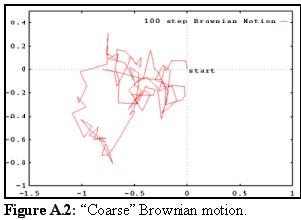
With Brownian motion, the moving object tends to meander a great deal on its path, frequently backtracking, and jumping from side to side. An example of the Brownian motion of a particle with a step size of standard deviation 0.1 is shown in figure A.2:
 One of the difficulties in simulating a system
like this is in deciding what level of detail
to use. As shown in figure A.2 above, the
motion is quite erratic, especially as each
of the small, linear paths represented in
the image is actually another small
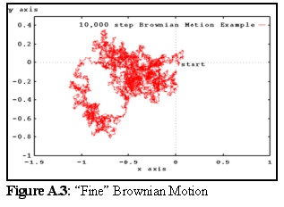
random walk. Figure A.3 shows the same
particle's path, but at a resolution of
10,000 steps, each with a distance of 0.01
standard deviations.
One of the difficulties in simulating a system
like this is in deciding what level of detail
to use. As shown in figure A.2 above, the
motion is quite erratic, especially as each
of the small, linear paths represented in
the image is actually another small
random walk. Figure A.3 shows the same
particle's path, but at a resolution of
10,000 steps, each with a distance of 0.01
standard deviations.
As these graphs show, Brownian motion is fractal in nature - the path becomes more and more convoluted as the scale is reduced. In reality, when considering the trajectories of molecules, the paths really do become almost straight lines at the picometer scale (some curvature may caused, especially in liquids, due to inter-molecular forces), but this is well below the level of the simulation. In order to make sure this collision simulation program is accurate enough, a step size must be picked that is small compared to the radius of the spheres being tested.
To simulate the problem domain, a series of tests were run. Since the problem was scalable, everything was measured in arbitrary size units. The standard deviation of the test point's movement was set to be 1 unit, which also sets the basic scale of the simulation - everything can now be measured either in "standard units" or equivalently in multiples of "one standard deviation".
The test was run for spheres sized 0.1 to 10 standard units in radius, and these were tested against interaction distances from 0 to 10 standard units in size. (As expected, and as is shown below, there were negligible interactions past about two standard deviations, or two "standard units", in distance.)
In all, 100,000 iterations (i.e. 100,000 different test points and spheres were used to test each radius and distance combination) for 20 different distances and 40 different sphere sizes. To simulate the "random walk" of the particle, rather than moving in one step of standard deviation 1, each sphere was moved in 10,000 steps of standard deviation .01, for the reasons explained above. This step size was chosen so that the resultant standard deviation of .01 units would be substantially smaller than the smallest radius tested, which was 0.1 units in size.
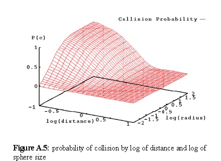
Despite the large number of individual steps (10,000 steps of standard deviation 0.01 units) the eventual standard deviation is the same (1 unit), and the step size is sufficiently smaller than the smallest radius tested, and thus accurately simulates the random walk nature of the particle's movement. The graphical results are presented below, with distance 1 equalling 1 unit (which is also 1 standard deviation), and sphere radius 1 that is likewise 1 unit (or 1 standard deviation) in size:
As can be seen in figure A.4, the function is, unsurprisingly, concentrated about large spheres and small distances. Slightly clearer are the same figures, presented in figure A.5 as a graph of probability against the log of distance and sphere size.
These numbers are used in the program whenever two objects come sufficiently close to each other (usually within three movement standard deviations or less) that they might possibly collide within the next time step. The probabilities above, scaled appropriately, are referred to via a lookup table, and a randomiser is used to determine whether a collision did, in fact, occur with the indicated probability.
The use of a lookup table ensures that, although computing the figures initially took some time (on the order of five hours), the speed of the program is unimpaired, since the time for finding the appropriate collision probability in the pre-calculated table is very small, and constant.
The raw data produced by the collision simulator are presented on the next two pages. The tables give the probability of collision, tabulated against the inter-sphere distances (across the top, measured in combined standard deviations of movement ), and the combined radii of the spheres, (also measured in standard deviations of movement ). (See page A.2 for a fuller explanation of the measurements used.)
Because the figures are derived from a probabilistic simulation, there is some inaccuracy. It must be remembered that each figure represents a trial of only 100,000 tests. This can be seen especially in the smaller numbers (i.e. at greater distances, or for smaller radii).
This can also be seen in the limiting case where the point and the sphere start at zero distance. In this case, it is theoretically certain (P = 1.0) that the point, moving in a Brownian manner, will collide with the sphere. Due to the discrete nature of the simulation though, this is only approximated in the results (see the "Distance Between Spheres" column for distance = 0 overleaf) which range from 0.447 for the smallest sphere with radius 0.0125 , to 0.996 for the largest, at 100 ).
This result for the tiny sphere (0.0125 ) is not surprising, since the "step size" of the Brownian motion was only 0.01 . More accurate figures could be obtained by simply decreasing the step size; however in practice it is unlikely (and undesirable) that simulation objects will be moving, on average, 100 times their size! Conversely, the figures (for this limiting case only) are within 5% of the theoretical limit once the sphere size is within about 1/8 of the RMS movement .
Collision Probabilities 1:
This page covers inter-sphere distances from 0.1 to 1 standard deviations.
Distance Between Spheres
| Radii | 0 | 0.1 | 0.125893 | 0.158489 | 0.199526 | 0.251189 | 0.316228 | 0.398107 | 0.501187 | 0.630957 | 0.794328 | 1 |
| 0.01 | ||||||||||||
| 0.012589 | 0.44689 | 0.06639 | 0.05475 | 0.04384 | 0.03718 | 0.02873 | 0.02221 | 0.01589 | 0.01128 | 0.00715 | 0.00391 | 0.00224 |
| 0.015849 | 0.55803 | 0.09506 | 0.07812 | 0.06415 | 0.05321 | 0.04191 | 0.03202 | 0.02298 | 0.01581 | 0.01049 | 0.00584 | 0.00322 |
| 0.019953 | 0.64968 | 0.12835 | 0.10693 | 0.08815 | 0.07289 | 0.05725 | 0.0445 | 0.03299 | 0.02222 | 0.01461 | 0.00815 | 0.00442 |
| 0.025119 | 0.72475 | 0.16737 | 0.13966 | 0.11672 | 0.09629 | 0.07681 | 0.05856 | 0.0443 | 0.02966 | 0.01932 | 0.01085 | 0.00595 |
| 0.031623 | 0.78301 | 0.21186 | 0.17792 | 0.14953 | 0.12384 | 0.09901 | 0.07555 | 0.05781 | 0.03865 | 0.0251 | 0.01437 | 0.00774 |
| 0.039811 | 0.82801 | 0.26128 | 0.222 | 0.18831 | 0.15557 | 0.12528 | 0.09599 | 0.07313 | 0.04979 | 0.03227 | 0.01863 | 0.00989 |
| 0.050119 | 0.86504 | 0.31539 | 0.27237 | 0.23102 | 0.19222 | 0.15527 | 0.12013 | 0.091 | 0.06243 | 0.04071 | 0.0236 | 0.01261 |
| 0.063096 | 0.89311 | 0.37442 | 0.32491 | 0.27826 | 0.23271 | 0.18923 | 0.14788 | 0.11164 | 0.07764 | 0.05047 | 0.02972 | 0.01555 |
| 0.079433 | 0.91571 | 0.43412 | 0.38098 | 0.32829 | 0.2766 | 0.22772 | 0.17908 | 0.13535 | 0.0951 | 0.06243 | 0.03697 | 0.01939 |
| 0.1 | 0.93387 | 0.49353 | 0.43859 | 0.38094 | 0.32434 | 0.26828 | 0.21339 | 0.16125 | 0.11448 | 0.07549 | 0.04561 | 0.0239 |
| 0.125893 | 0.94766 | 0.55135 | 0.49442 | 0.4342 | 0.3729 | 0.31157 | 0.24897 | 0.18991 | 0.13628 | 0.09032 | 0.05506 | 0.02924 |
| 0.158489 | 0.95875 | 0.60427 | 0.54781 | 0.48711 | 0.42096 | 0.35498 | 0.28673 | 0.22022 | 0.16027 | 0.10728 | 0.06606 | 0.03503 |
| 0.199526 | 0.96723 | 0.65385 | 0.59804 | 0.53721 | 0.46981 | 0.39946 | 0.32723 | 0.25455 | 0.18567 | 0.12615 | 0.07745 | 0.04149 |
| 0.251189 | 0.97405 | 0.69691 | 0.64453 | 0.58393 | 0.51782 | 0.44404 | 0.36708 | 0.28932 | 0.21401 | 0.14693 | 0.09075 | 0.04861 |
| 0.316228 | 0.97944 | 0.73578 | 0.68633 | 0.62748 | 0.56134 | 0.48704 | 0.40812 | 0.32511 | 0.24397 | 0.16959 | 0.10579 | 0.05756 |
| 0.398107 | 0.98292 | 0.7692 | 0.7231 | 0.6681 | 0.60344 | 0.52972 | 0.44831 | 0.3617 | 0.27553 | 0.19402 | 0.12268 | 0.06697 |
| 0.501187 | 0.9855 | 0.79776 | 0.75557 | 0.70324 | 0.64044 | 0.56897 | 0.48756 | 0.39797 | 0.30692 | 0.21969 | 0.14027 | 0.07776 |
| 0.630957 | 0.98781 | 0.82199 | 0.78313 | 0.73454 | 0.67494 | 0.6055 | 0.52505 | 0.43399 | 0.33802 | 0.24582 | 0.15998 | 0.08961 |
| 0.794328 | 0.98956 | 0.84161 | 0.8054 | 0.76047 | 0.70418 | 0.63744 | 0.55823 | 0.46643 | 0.37007 | 0.27185 | 0.18003 | 0.10231 |
| 1 | 0.9909 | 0.85836 | 0.82464 | 0.78253 | 0.73106 | 0.6658 | 0.58902 | 0.49766 | 0.39944 | 0.29826 | 0.20036 | 0.11604 |
| 1.25893 | 0.99199 | 0.87199 | 0.84063 | 0.80085 | 0.75155 | 0.68982 | 0.61549 | 0.526 | 0.42683 | 0.32335 | 0.22017 | 0.12976 |
| 1.58489 | 0.9928 | 0.88279 | 0.85371 | 0.81598 | 0.76954 | 0.70965 | 0.63804 | 0.55061 | 0.4514 | 0.34609 | 0.23959 | 0.14401 |
| 1.99526 | 0.99334 | 0.89143 | 0.86405 | 0.82876 | 0.78406 | 0.72755 | 0.6575 | 0.57154 | 0.47346 | 0.36669 | 0.25754 | 0.15708 |
| 2.51189 | 0.99386 | 0.89851 | 0.87244 | 0.83896 | 0.79642 | 0.74215 | 0.67398 | 0.58923 | 0.49139 | 0.38523 | 0.27329 | 0.16948 |
| 3.16228 | 0.99425 | 0.90406 | 0.87896 | 0.8471 | 0.80597 | 0.75351 | 0.68759 | 0.60396 | 0.50697 | 0.40098 | 0.2882 | 0.18058 |
| 3.98107 | 0.99459 | 0.90854 | 0.88472 | 0.85371 | 0.81315 | 0.76251 | 0.69835 | 0.61642 | 0.52031 | 0.41418 | 0.30031 | 0.19065 |
| 5.01187 | 0.99484 | 0.91237 | 0.88925 | 0.8592 | 0.81969 | 0.77028 | 0.70729 | 0.62634 | 0.53149 | 0.42514 | 0.31064 | 0.19927 |
| 6.30957 | 0.99503 | 0.91505 | 0.89271 | 0.86386 | 0.82481 | 0.7762 | 0.71436 | 0.63499 | 0.54043 | 0.43394 | 0.3193 | 0.20668 |
| 7.94328 | 0.99519 | 0.91736 | 0.89542 | 0.86705 | 0.829 | 0.78117 | 0.71987 | 0.64172 | 0.54771 | 0.44126 | 0.32671 | 0.21283 |
| 10 | 0.99533 | 0.91924 | 0.8979 | 0.87006 | 0.83225 | 0.78483 | 0.72431 | 0.64738 | 0.55403 | 0.44779 | 0.3328 | 0.2177 |
| 12.5893 | 0.99542 | 0.92083 | 0.8996 | 0.87214 | 0.83508 | 0.78808 | 0.72804 | 0.65189 | 0.55904 | 0.45277 | 0.33726 | 0.22223 |
| 15.8489 | 0.99552 | 0.92188 | 0.90076 | 0.87387 | 0.83731 | 0.79069 | 0.73107 | 0.65542 | 0.56287 | 0.45676 | 0.3412 | 0.22582 |
| 19.9526 | 0.99562 | 0.92273 | 0.9019 | 0.87531 | 0.83891 | 0.79279 | 0.73331 | 0.65807 | 0.56583 | 0.46006 | 0.3443 | 0.22873 |
| 25.1189 | 0.99566 | 0.92334 | 0.90281 | 0.87654 | 0.84042 | 0.79437 | 0.73517 | 0.66052 | 0.56815 | 0.46273 | 0.34669 | 0.23082 |
| 31.6228 | 0.99571 | 0.92401 | 0.9035 | 0.87741 | 0.84153 | 0.79581 | 0.73689 | 0.66235 | 0.57024 | 0.46476 | 0.34899 | 0.23251 |
| 39.8107 | 0.99576 | 0.92441 | 0.90413 | 0.87793 | 0.84245 | 0.79679 | 0.73832 | 0.66373 | 0.57199 | 0.46631 | 0.35056 | 0.23385 |
| 50.1187 | 0.99576 | 0.92476 | 0.90461 | 0.87834 | 0.84291 | 0.79774 | 0.73932 | 0.66507 | 0.57311 | 0.46754 | 0.35179 | 0.23506 |
| 63.0957 | 0.99576 | 0.92503 | 0.90496 | 0.87875 | 0.84341 | 0.79835 | 0.74002 | 0.66595 | 0.57391 | 0.46872 | 0.35265 | 0.23593 |
| 79.4328 | 0.99578 | 0.92529 | 0.90522 | 0.87906 | 0.84381 | 0.79887 | 0.74076 | 0.66657 | 0.57491 | 0.46971 | 0.35354 | 0.2367 |
| 100 | 0.99578 | 0.92548 | 0.90543 | 0.87935 | 0.84407 | 0.79934 | 0.74123 | 0.66715 | 0.57554 | 0.4704 | 0.35412 | 0.23731 |
Collision Probabilities 2:
This page covers inter-sphere distances from 1 to 10 standard deviations. (The '1' column is repeated for clarity):
Distance Between Spheres
| Radii | 1 | 1.25893 | 1.58489 | 1.99526 | 2.51189 | 3.16228 | 3.98107 | 5.01187 | 6.30957 | 7.94328 | 10 |
| 0.01 | |||||||||||
| 0.012589 | 0.00224 | 0.00094 | 0.0003 | 0 | 0 | 0 | 0 | 0 | 0 | 0 | 0 |
| 0.015849 | 0.00322 | 0.00126 | 0.00046 | 0 | 0 | 0 | 0 | 0 | 0 | 0 | 0 |
| 0.019953 | 0.00442 | 0.00172 | 0.00065 | 0.0001 | 1.00E-05 | 0 | 0 | 0 | 0 | 0 | 0 |
| 0.025119 | 0.00595 | 0.00238 | 0.00088 | 0.00018 | 1.00E-05 | 0 | 0 | 0 | 0 | 0 | 0 |
| 0.031623 | 0.00774 | 0.00316 | 0.00117 | 0.00023 | 2.00E-05 | 0 | 0 | 0 | 0 | 0 | 0 |
| 0.039811 | 0.00989 | 0.00406 | 0.00144 | 0.00027 | 2.00E-05 | 0 | 0 | 0 | 0 | 0 | 0 |
| 0.050119 | 0.01261 | 0.00514 | 0.0018 | 0.0003 | 2.00E-05 | 0 | 0 | 0 | 0 | 0 | 0 |
| 0.063096 | 0.01555 | 0.00647 | 0.00221 | 0.00036 | 2.00E-05 | 0 | 0 | 0 | 0 | 0 | 0 |
| 0.079433 | 0.01939 | 0.00803 | 0.00267 | 0.00051 | 2.00E-05 | 0 | 0 | 0 | 0 | 0 | 0 |
| 0.1 | 0.0239 | 0.00998 | 0.00322 | 0.00061 | 4.00E-05 | 0 | 0 | 0 | 0 | 0 | 0 |
| 0.125893 | 0.02924 | 0.01215 | 0.00394 | 0.00071 | 7.00E-05 | 0 | 0 | 0 | 0 | 0 | 0 |
| 0.158489 | 0.03503 | 0.01487 | 0.00477 | 0.00093 | 0.0001 | 0 | 0 | 0 | 0 | 0 | 0 |
| 0.199526 | 0.04149 | 0.018 | 0.00573 | 0.00108 | 0.00011 | 1.00E-05 | 0 | 0 | 0 | 0 | 0 |
| 0.251189 | 0.04861 | 0.02167 | 0.00669 | 0.00129 | 0.00013 | 1.00E-05 | 0 | 0 | 0 | 0 | 0 |
| 0.316228 | 0.05756 | 0.02573 | 0.00789 | 0.00154 | 0.00016 | 1.00E-05 | 0 | 0 | 0 | 0 | 0 |
| 0.398107 | 0.06697 | 0.02996 | 0.00953 | 0.00177 | 0.0002 | 1.00E-05 | 0 | 0 | 0 | 0 | 0 |
| 0.501187 | 0.07776 | 0.03507 | 0.01127 | 0.00215 | 0.00023 | 1.00E-05 | 0 | 0 | 0 | 0 | 0 |
| 0.630957 | 0.08961 | 0.04122 | 0.01355 | 0.00263 | 0.00027 | 1.00E-05 | 0 | 0 | 0 | 0 | 0 |
| 0.794328 | 0.10231 | 0.04772 | 0.0161 | 0.00318 | 0.00034 | 1.00E-05 | 0 | 0 | 0 | 0 | 0 |
| 1 | 0.11604 | 0.05471 | 0.01892 | 0.00382 | 0.00046 | 2.00E-05 | 0 | 0 | 0 | 0 | 0 |
| 1.25893 | 0.12976 | 0.06189 | 0.02202 | 0.00444 | 0.00052 | 2.00E-05 | 0 | 0 | 0 | 0 | 0 |
| 1.58489 | 0.14401 | 0.06959 | 0.02499 | 0.00522 | 0.00062 | 2.00E-05 | 0 | 0 | 0 | 0 | 0 |
| 1.99526 | 0.15708 | 0.07778 | 0.0283 | 0.00603 | 0.00074 | 2.00E-05 | 0 | 0 | 0 | 0 | 0 |
| 2.51189 | 0.16948 | 0.08504 | 0.03178 | 0.00695 | 0.00085 | 2.00E-05 | 0 | 0 | 0 | 0 | 0 |
| 3.16228 | 0.18058 | 0.09222 | 0.03529 | 0.0078 | 0.00095 | 2.00E-05 | 0 | 0 | 0 | 0 | 0 |
| 3.98107 | 0.19065 | 0.09854 | 0.03852 | 0.00872 | 0.00102 | 2.00E-05 | 0 | 0 | 0 | 0 | 0 |
| 5.01187 | 0.19927 | 0.10402 | 0.0412 | 0.00959 | 0.00113 | 2.00E-05 | 0 | 0 | 0 | 0 | 0 |
| 6.30957 | 0.20668 | 0.10885 | 0.04399 | 0.01056 | 0.00121 | 4.00E-05 | 0 | 0 | 0 | 0 | 0 |
| 7.94328 | 0.21283 | 0.11311 | 0.04623 | 0.01137 | 0.00128 | 5.00E-05 | 0 | 0 | 0 | 0 | 0 |
| 10 | 0.2177 | 0.11713 | 0.04823 | 0.01197 | 0.00141 | 5.00E-05 | 0 | 0 | 0 | 0 | 0 |
| 12.5893 | 0.22223 | 0.11979 | 0.04972 | 0.01252 | 0.00147 | 7.00E-05 | 0 | 0 | 0 | 0 | 0 |
| 15.8489 | 0.22582 | 0.12225 | 0.05104 | 0.0131 | 0.00159 | 7.00E-05 | 0 | 0 | 0 | 0 | 0 |
| 19.9526 | 0.22873 | 0.1243 | 0.05208 | 0.01359 | 0.00164 | 8.00E-05 | 0 | 0 | 0 | 0 | 0 |
| 25.1189 | 0.23082 | 0.12601 | 0.05305 | 0.01393 | 0.0017 | 8.00E-05 | 0 | 0 | 0 | 0 | 0 |
| 31.6228 | 0.23251 | 0.12733 | 0.05379 | 0.01422 | 0.00182 | 8.00E-05 | 0 | 0 | 0 | 0 | 0 |
| 39.8107 | 0.23385 | 0.12842 | 0.05436 | 0.01455 | 0.00187 | 8.00E-05 | 0 | 0 | 0 | 0 | 0 |
| 50.1187 | 0.23506 | 0.12915 | 0.055 | 0.01477 | 0.00189 | 8.00E-05 | 0 | 0 | 0 | 0 | 0 |
| 63.0957 | 0.23593 | 0.12995 | 0.05545 | 0.01496 | 0.00191 | 8.00E-05 | 0 | 0 | 0 | 0 | 0 |
| 79.4328 | 0.2367 | 0.13047 | 0.05577 | 0.0151 | 0.00194 | 8.00E-05 | 0 | 0 | 0 | 0 | 0 |
| 100 | 0.23731 | 0.13093 | 0.05604 | 0.01523 | 0.00194 | 8.00E-05 | 0 | 0 | 0 | 0 | 0 |
While an analytic solution would be desirable, in its absence the probabilities of collision of objects have been obtained by simply simulating a sphere and a randomly moving test point many thousands of times.
The results of this simulation have been incorporated into a data file which the modelling program reads when it starts running, allowing it to quickly determine the probability of collision for any pair of objects being simulated.
Index |
Last Chapter |
Next Appendix |
1. This is a well known lemma; e.g. Bhattacharyya, G.K. & Johnson, R.A, (1977) Statistical Concepts and Methods, John Wiley & Sons, pp 202